Convergent-divergent nozzle
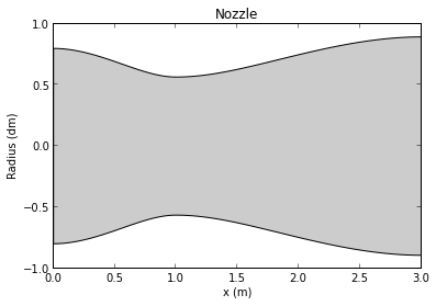
Statement: Determine the steady flow within the convergent-divergent nozzle, geometrically defined by
for the operating condition in which the nozzle discharges in the atmosphere and is supplied with a stagnation pressure P_0 = 2 atm and a stagnation temperature T0 = 300 °C.
Algorithm
Temptative algorithm: given nozzle geometry \(A(x)\), ambient pressure \(p_A\) and inlet stagnation conditions \(p_0\) and \(T_0\),
We are discharging to the atmosphere, therefore the back pressure \(p_B\) is the given ambient pressure.
Supose chocked flow, hence minimal area \(A_t\) is critical area \(A^*\).
Compute \(M_e\) both subsonic and supersonic, using the Mach number-area ratio relation.
Compute subsonic \(p_{e3}\) and supersonic \(p_{e6}\) pressure at the exit using isentropic Mach number relations and inlet stagnation pressure.
Compare \(p_B\) with \(p_{e3}\) and \(p_{e6}\):
If \(p_{e3} \lt p_B\), fully subsonic flow, no sonic conditions at the throat.
If \(p_B \leq p_{e3}\), chocked flow.
…
Computations
[1]:
%pylab inline

# Import necessary packages
import numpy as np
import scipy as sp

from scipy import constants, optimize

import matplotlib.pyplot as plt
Welcome to pylab, a matplotlib-based Python environment [backend: module://IPython.zmq.pylab.backend_inline].
For more information, type 'help(pylab)'.
[2]:
from skaero.gasdynamics import isentropic, shocks
[3]:
# 0. Given conditions
# Taken from exercises 2 and 18

# Parameters
gamma = g = 1.4
R = 287.04  # J / (kg · K)
p_amb = 1 * sp.constants.atm  # Pa

# Inlet conditions
p_0 = 2.0 * sp.constants.atm  # Pa
T_0 = sp.constants.C2K(300.0)  # K

# Longitudinal axis of the nozzle
x = np.linspace(0, 3, 151)
[4]:
# Geometry of the nozzle
def A(x):
    """Cross sectional area of the nozzle, in m^2.

    Notice that this function also contains a couple of workarounds
    to circunvent some odd behaviour of numpy.piecewise.
    """
    def A_1(x):
        return (2.0 * x ** 3 - 3.0 * x ** 2 + 2.0) / 100

    def A_2(x):
        return (-3.0 * x ** 3 / 8.0 + 9.0 * x ** 2 / 4.0 - 27.0 * x / 8.0 + 5.0 / 2.0) / 100

    x = np.asarray(x, dtype=float)
    # For avoiding np.piecewise bug
    if not x.shape:
        x = np.asarray([x])

    result = np.piecewise(x, [(0.0 <= x) & (x < 1.0), (1.0 <= x) & (x <= 3.0)], [A_1, A_2])
    if len(result) == 1:
        result = result[0]

    return result

radius = np.sqrt(A(x) / np.pi) * 10  # dm

# Plot nozzle shape
nozzle = plt.fill_between(x, radius, -radius, facecolor="#cccccc")
plt.xlim(0, 3)
plt.title("Nozzle")
plt.xlabel("x (m)")
plt.ylabel("Radius (dm)")
[4]:
<matplotlib.text.Text at 0x7fe7d80ade10>
[5]:
# 1. Back pressure pB is ambient pressure
p_B = p_amb
[6]:
# 2. Find minimum area in domain
A_e = A(x[-1])  # m^2
A_c = np.min(A(x))  # m^2
[7]:
# 3. Compute subsonic and supersonic Mach number at the exit
fl = isentropic.IsentropicFlow(gamma=g)
M_e_sub, M_e_sup = isentropic.mach_from_area_ratio(fl, A_e / A_c)

print(A_e / A_c)
print(M_e_sub, M_e_sup)
2.5
0.23954284305818874 2.44276484552
/home/juanlu/.local/lib/python3.3/site-packages/skaero/gasdynamics/isentropic.py:150: RuntimeWarning: divide by zero encountered in double_scalars
  ((self.gamma + 1) / (2 * (self.gamma - 1))) / M
[8]:
# 4. Compute pressure limit values
from IPython.core.display import Latex

Latex(r"\[\frac{p_0}{p} = (1 + \frac{\gamma - 1}{2} M^2)^{\gamma / (\gamma - 1)}\]")
[8]:
[9]:
# Isentropic limit subsonic and supersonic solutions
p_e3 = p_0 * fl.p_p0(M_e_sub)
p_e6 = p_0  * fl.p_p0(M_e_sup)

print("Exit pressure of the limit isentropic solutions")
print(p_e3, p_e6)
Exit pressure of the limit isentropic solutions
194716.088639 12966.4263803
[10]:
# Normal shock at the exit of the nozzle
# ...
[11]:
# Isentropic pressure solutions
M_isen = np.empty((len(x), 2))
for i in range(len(x)):
    M_isen[i] = isentropic.mach_from_area_ratio(fl, A(x[i]) / A_c)

# Subsonic isentropic limit solution
M_isen_sub = M_isen[np.arange(len(x)), np.zeros(len(x), dtype=int)]
p_isen_sub = fl.p_p0(M_isen_sub)

# Supersonic isentropic solution
i_c = np.argmin(A(x))
mask = np.zeros(len(x), dtype=int)
mask[i_c:] = 1
M_isen_sup = M_isen[np.arange(len(x)), mask]
p_isen_sup = fl.p_p0(M_isen_sup)
[12]:
# 5. Discriminate flow
# TODO: I need to compute also the shock inside nozzle, overexpanded, properly expanded
# and underexpanded cases.
if p_B > p_e3:
    print("Fully subsonic flow")
elif p_B <= p_e3:
    print("Chocked flow")
Chocked flow
[13]:
# Given normal shock location, return pressure
def pe_p0_from_shock_location(A_loc_ratio, A_e_ratio):
    # 1. Compute M_1
    M_1 = isentropic.mach_from_area_ratio(fl, A_loc_ratio)[1]
    # 2. Compute M_2
    ns = shocks.NormalShock(M_1, gamma)
    M_2 = ns.M_2
    # 3. Compute A_2 over A_2^*
    a2_a2c = fl.A_Astar(M_2)
    # 4. Compute A_e / A_2^*
    ae_a2c = A_e_ratio / A_loc_ratio * a2_a2c
    # 5. Compute M_e
    M_e = isentropic.mach_from_area_ratio(fl, ae_a2c)[0]
    # 6. Compute p_e over p_0e
    p0e_pe = 1 / fl.p_p0(M_e)
    # 7. Compute p_02 over p_2
    p02_p2 = 1 / fl.p_p0(M_2)
    # 8. Compute p_2 over p_1
    p2_p1 = ns.p2_p1
    # 9. Compute p_01 over p_1
    p01_p1 = 1 / fl.p_p0(M_1)
    # 10. Compute p_02 over p_01
    p02_p01 = p02_p2 * p2_p1 * 1 / p01_p1
    # 11. Compute p_e over p_0
    pe_p0 = 1 / p0e_pe * p02_p01
    return pe_p0


#print(p_e_from_shock_location(2.0, 3.0))  # Anderson example 5.6, it works
def F(A_loc_ratio, A_e_ratio, pe_p0):
    return pe_p0_from_shock_location(A_loc_ratio, A_e_ratio) - pe_p0

#print(sp.optimize.brentq(F, 1.0, 3.0, args=(3.0, 0.5)))  # Anderson example 5.7, works
#print(F(2.3397, 3.0, 0.5))  # 5.84275393312e-06

A_shock = sp.optimize.brentq(F, 1.0, 3.0, args=(A_e / A_c, p_B / p_0))
print("Location of the normal shock")
print(A_shock * A_c)
Location of the normal shock
0.0222720756212
[14]:
# Find corresponding index
def find_nearest_index(a, a0):
    """Element in nd array a closest to the scalar value a0.

    See http://stackoverflow.com/a/10465997/554319

    """
    idx = np.abs(a - a0).argmin()
    return idx


Area = A(x)
i_s = find_nearest_index(Area, A_shock * A_c)
x[i_s]
[14]:
2.46
[15]:
# Compute pressure along nozzle axis
p_ratio = np.empty_like(x)

# Isentropic portion
p_ratio[:i_s] = p_isen_sup[:i_s]

# Portion behind the shock
# 1. Compute M_1
M_1 = isentropic.mach_from_area_ratio(fl, A_shock)[1]
# 2. Compute M_2
ns = shocks.NormalShock(M_1, gamma)
M_2 = ns.M_2
# 3. Compute A_2 over A_2^*
a2_a2c = fl.A_Astar(M_2)
A_c2 = A_shock * A_c / a2_a2c

M_post = np.empty_like(x[i_s:])
for i in range(len(x[i_s:])):
    M_post[i] = isentropic.mach_from_area_ratio(fl, A(x[i_s + i]) / A_c2)[0]

print(M_post)
p_ratio[i_s:] = fl.p_p0(M_post)
[ 0.53107106  0.52502108  0.51928679  0.51385348  0.50870794  0.50383834
  0.49923405  0.49488553  0.49078421  0.48692242  0.48329332  0.47989083
  0.47670958  0.47374485  0.47099257  0.46844926  0.46611202  0.46397849
  0.46204687  0.4603159   0.45878484  0.45745348  0.45632216  0.45539176
  0.45466371  0.45414004  0.45382338  0.45371699]
[16]:
# Mach number distribution
M = np.zeros_like(x)
M[:i_s] = M_isen_sup[:i_s]
M[i_s:] = M_post
[17]:
# Plot whole solution
fig = plt.figure(figsize=(6, 8))
#ax_nozzle = fig.add_subplot(211)
#ax_nozzle.fill_between(x, radius, -radius, facecolor="#cccccc")
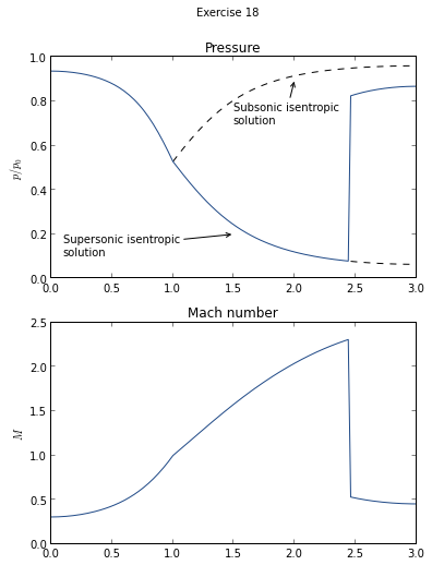
ax_press = fig.add_subplot(211)
ax_press.plot(x[i_c:], p_isen_sub[i_c:], 'k--', x[i_s:], p_isen_sup[i_s:], 'k--')
ax_press.annotate(s="Subsonic isentropic\nsolution", xy=(2.0, 0.9), xytext=(1.5, 0.7), arrowprops=dict(arrowstyle = "->"))
ax_press.annotate(s="Supersonic isentropic\nsolution", xy=(1.5, 0.2), xytext=(0.1, 0.1), arrowprops=dict(arrowstyle = "->"))
ax_press.set_ylabel(r"$p / p_0$")
ax_press.plot(x, p_ratio)
ax_press.set_title("Pressure")
ax_mach = fig.add_subplot(212)
ax_mach.plot(x, M)
ax_mach.set_ylabel("$M$")
ax_mach.set_title("Mach number")
fig.suptitle("Exercise 18")
fig.savefig("exercise_18.png", dpi=100)
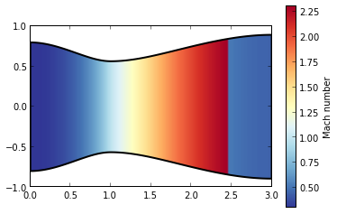
[18]:
import matplotlib.cm as cm

xx, MM = np.meshgrid(x, M)
fig = plt.figure()
ax = fig.add_subplot(111)
im = ax.imshow(MM.transpose(), extent=(0, 3, -1, 1), cmap=cm.RdYlBu_r)
cb = fig.colorbar(im)
cb.set_label("Mach number")

import matplotlib.patches as patches

patch = patches.PathPatch(nozzle.get_paths()[0], fc='none', lw=2)
ax.add_patch(patch)
im.set_clip_path(patch)
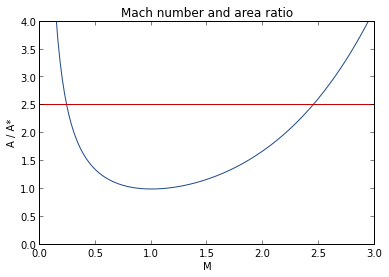
This is the Mach number-area ratio relation.
[19]:
M_range = np.linspace(0, 4, 201)
plt.plot(M_range, fl.A_Astar(M_range))
plt.plot(x, A_e / A_c * np.ones_like(x))
plt.xlim(0, 3)
plt.ylim(0, 4)
plt.title("Mach number and area ratio")
plt.xlabel("M")
plt.ylabel("A / A*")
/home/juanlu/.local/lib/python3.3/site-packages/skaero/gasdynamics/isentropic.py:150: RuntimeWarning: divide by zero encountered in true_divide
  ((self.gamma + 1) / (2 * (self.gamma - 1))) / M
[19]:
<matplotlib.text.Text at 0x7fe7c3cd85d0>
[19]: